GridSFM: A new, small foundation model for the electric grid

Microsoft releases a lightweight foundation model that can predict AC optimal power flow in milliseconds, boosting efficiency and unlocking cost savings in grid analysis.

Microsoft introduces GridSFM, a small foundation model for solving AC optimal power flow (AC-OPF) problems in transmission power grids. This follows our earlier release of a U.S.-based open transmission-topology dataset that powers GridSFM.

Power grids face increasing strain from surging demand, the need to integrate renewable energy sources, transportation electrification, and extreme weather events. Across all these challenges, the core question is the same: what are the optimal operating points that keep the grid functioning under each new condition?

Answering this requires solving AC optimal power flow (AC‑OPF), a complex, non-convex optimization problem that computes the cheapest generator dispatch (how much each generator produces) that meets demands while respecting power flow physics, voltage limits, thermal constraints, and stability requirements, and underpins core power system operations including reliability, real-time dispatch, market clearing, and contingency analysis. These decisions directly govern outcomes at the scale of up $20 billion per year in congestion costs (opens in new tab) and multi‑terawatt‑hour renewable curtailment (opens in new tab) (lost renewable energy due to congestion), making both economic efficiency and grid reliability highly sensitive to how well these operating points are found. However, AC‑OPF is computationally expensive: power utility scale grid can take up to hours solve, forcing a trade-off between solving a small number of carefully selected scenarios or relying on approximations that ignore critical physics, which can misestimate power flows and binding constraints and lead to suboptimal dispatch and degraded reliability under stressed conditions.

To address this limitation, we introduce GridSFM, a single neural network that approximates AC‑OPF in milliseconds across grids ranging from 500 to 80,000 buses. It takes standard AC‑OPF inputs (grid topology, generator and load specifications, transmission line constraints) and produces an operating point and a feasibility verdict (whether the system satisfies all physical and operational constraints). By removing the compute bottleneck, GridSFM makes it possible to evaluate orders of magnitude more scenarios in real time, enabling more informed decisions and shifting grid operations from reactive response to proactive optimization.

In this initial release we offer two tiers:

• GridSFM-Open for research-scale grids up to 4,000 buses.
• GridSFM-Premier for production-scale systems up to 80,000 buses.

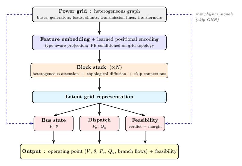
The model is built as a block-structured discrete neural operator (Figure 1), representing each grid as a directed graph, with buses (connection points in the grid) and generators as vertices, and transmission and AC lines as edges. It is trained using both solver supervision, where reference solutions are generated using the AC-OPF solver (IPOPT in PowerModels.jl (opens in new tab)), and physics-based constraints that penalize violations of fundamental physical laws such as Kirchhoff’s voltage and current laws, as well as operating constraints like thermal limits. This enables the model to learn from both feasible and infeasible regimes. Most learning-based AC-OPF surrogates train one model per grid on a narrow distribution (opens in new tab). GridSFM takes the opposite approach: in this release a single model trained across 150+ base grid topologies (network structures) and roughly half a million scenarios spanning varying load profiles, multi-element outages, line-rating derates, voltage-bound tightening, and different generator cost coefficients, so the model is forced to generalize rather than memorize. Across the 54-grid mix test scenarios for GridSFM-Open, our model achieves a median cost gap of 2.23% vs solver ground truth labels (mean 3.41%; <5% gap on 83 % of scenarios). When more precision is needed, GridSFM’s prediction also serves as a warm start seed for traditional numerical solvers, GridSFM-seeded-warm beats cold solve by 1.66× geometric mean across the same test scenarios and beats the industry-standard DC-OPF warm-start by 1.59× geomean (per-grid breakdown and full white-paper analysis to follow).  Geometric mean, otherwise known as the multiplicative average, is used here since it is more robust to outliers. Our model also demonstrates the ability to adapt to new grids with just a handful of fine-tune scenarios.

What it enables

A common pattern in grid operations and planning is having to choose between solving a small, hand-picked set of scenarios accurately with full AC-OPF or running thousands of scenarios through a faster approximation that drops parts of the physics. For example, a commonly used tool is the DC-OPF approximation, a linearized version that assumes flat voltage magnitudes and small angle differences and ignores reactive power and losses. DC-approximation solves in seconds what takes full AC minutes to hours, which is why most contingency screens, market-clearing pre-stages, and planning sweeps run on DC-approximation today. The cost is real: DC-approximation ignores voltage and reactive constraints entirely, and its dispatch cost can run >10% off the AC optimum on stressed scenarios (with worst-case grids out past 20% in our test benchmark).

GridSFM is designed as a drop-in alternative to DC-approximation in that fast approximation slot, and unlike most existing AC-OPF neural surrogates, which require a fresh training run for every new topology, GridSFM generalizes across grids in its supported size range without per-topology retraining, so it slots in as universally as DC-approximation. Especially when compared with DC-OPF, GridSFM has three concrete advantages:

• Same accuracy class as DC-approximation on standalone dispatch cost. GridSFM and DC fall within the same per-scenario cost-gap distribution (§2 / Figure 6), with complementary failure modes: DC fails on grids where its no-loss / no-reactive linearization is structurally wrong; GridSFM fails on grids outside its training distribution. The two limitations close along orthogonal axes. DC’s ceiling is fixed by the linearization, whereas GridSFM’s tail closes with more training data.
• 1,000× faster than a full AC solver and approximately 100× faster than DC-approximation at the inference step, fast enough to sweep thousands of contingencies (e.g., line or generator outages) in minutes on a single commodity GPU.
• A real AC operating point, not a linear approximation. GridSFM produces voltages and reactive power, so the same prediction can be handed to a traditional numerical solver as an AC warm-start, opening a workflow DC-approximation cannot.

1. Feasibility screening: stress-score triage

A scenario is infeasible when no dispatch satisfies all constraints simultaneously: the requested load cannot be served within voltage bounds, thermal limits or generator capacities. Operationally, infeasibility is the most consequential failure signal: the requested operating condition cannot be served at all, and the response is intervention (load shedding, redispatch, relaxing thermal limits). It is also the most expensive class of scenario to screen, because the solver only learns a scenario is infeasible after iterating to non-convergence: each infeasible case costs a full solver run, often longer than a feasible one. Sweeping thousands of contingencies or stress cases to identify the infeasible ones is therefore one of the worst-case budgets in any planning workflow.

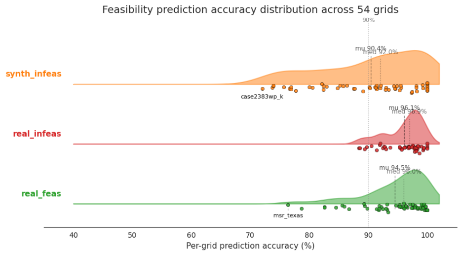
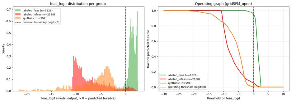
GridSFM addresses this with a per-scenario stress score trained jointly with the dispatch head. We evaluate the score on three classes of scenarios on each grid: real-feas are scenarios the AC-OPF solver successfully converged on (i.e., genuinely feasible operating points), real-infeas are scenarios the solver failed to converge on (genuinely infeasible operating points), and synth-infeas are feasible base points we deliberately perturbed to violate a specific constraint (voltage squeeze, thermal bottleneck, angle tightening, or DC-thermal congestion). Across the 54-grid test scenarios, the stress score’s per-grid binary accuracy is broadly uniform across classes: real-feas (green) mean 94.5%, real-infeas (red) mean 96.1%, synth-infeas (orange) mean 90.4%. Most grids cluster within a few points of the means; outliers below 80% are the same hard grids that show up in cost-gap analysis below.

Drilling into a case study. Let’s zoom into a single representative grid, the Texas2k summer-peak grid (opens in new tab), to show how the learned representation separates feasibility and ROC for predicting.

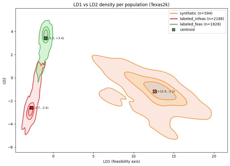
Representation. Figure 3 visualizes the model’s learned representation of each Texas2k scenario. We project the per-graph representation (128-dimensional) onto two axes (LD1, LD2) chosen to maximally separate the scenario classes: real-feasible, real-infeasible, and synthetic-infeasible. Squeezing 128 dimensions into 2 inevitably loses information, so this view exaggerates apparent overlap: classes that look mixed here may still be cleanly separable in the full 128-dimensional space the model uses. The shaded cloud shows where graphs of each class concentrate, and the cross at the center of each cloud marks the class centroid, the average position of all graphs of that class. Centroids that sit far apart mean the model treats those classes as clearly distinguishable. Where two shaded clouds overlap, the model is producing similar embeddings for graphs with different labels.

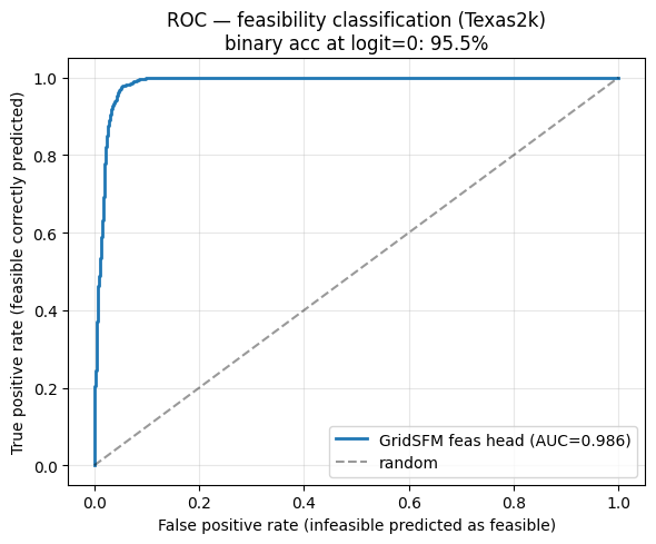
Operation and ROC. The score itself is continuous and ranking-calibrated. Figure 4 shows the ROC over its test mix: AUC = 0.986. At the natural operating point the same score, thresholded as a binary classifier, yields 95.5% accuracy. Per-mode detection at that threshold is 99–100% on the three perturbation modes that drive a constraint cleanly past its limit.

Triage cutoff. For routing scenarios into action buckets, Figure 5 shows the stress-score distribution per population. Operators pick the cutoff that matches their workflow: very-confident feasibles pass through to indicative dispatch; very-confident-stressed scenarios are flagged for engineering review; the borderline middle band is sent to the solver for verification. The cutoff sets the balance between solver budget and screening miss-rate.

2. GridSFM as a fast approximation

GridSFM’s prediction can be used in two ways without producing an exact AC-OPF solution from scratch: as a standalone dispatch and cost estimate, or as the initial guess (warm-start) for an exact numerical solver. We compare both against the same two reference points throughout: full AC-OPF (the ground-truth optimum) and DC-approximation (the established fast baseline). All numbers below come from the same test set of 54 grids scenarios GridSFM-Open, with solver solve_time measured per scenario under single-core CPU pinning.

Standalone cost estimate

When an exact solver round-trip is not required, GridSFM’s predicted dispatch can be costed directly. In our test set, GridSFM-Open and DC-approximation fall in the same accuracy class: comparable means (DC 2.80%, GridSFM 3.41%), comparable medians (DC 1.81% vs GridSFM 2.23%), and overlapping per-scenario distributions across two decades of cost gap (Figure 6). They have complementary failure modes rather than one dominating the other.

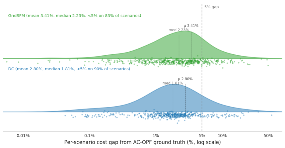
Both distributions look the same in shape: a single peak in the 2–3% gap range, with the bulk of scenarios under 5% and a small tail of outliers extending out into the >25% range. The outlier tails come from different sources: DC fails on grids where its no-reactive linearization is structurally wrong (case1803_snem and a handful of meshed transmission grids); GridSFM’s outliers are concentrated on a few of our open sourced grids whose AC-OPF reference itself required additional constraint relaxation to become feasible (opens in new tab), so the ground-truth target on those grids is noisier and the gap partly reflects reference-side instability. The two limitations close along orthogonal axes: DC’s ceiling is fixed by the linearization and does not improve with more data or compute; GridSFM’s tail closes with cleaner reference labels and more training data on those grid families.

The differentiating value of GridSFM is therefore not the standalone cost number, but that GridSFM produces a full AC operating point including voltages and reactive power. This allows operators to directly assess the state of the grid. This is important since the feasibility and security of a system is often determined by the voltage and reactive power limits, but neither are considered in DC-OPF.  At the same time, the operating point also enables the warm-start workflow, as we describe next.

Warm-start handoff

An AC-OPF solver works by iteratively refining an initial guess of the operating point until the optimality conditions are satisfied, and the number of refinement iterations it needs depends directly on how close the initial guess starts to the true optimum: a poor starting point can require thousands of iterations, a near-optimal one only a couple. A cold start (also known as a flat start) sets voltage magnitude to 1.0 per unit and angle to zero  on every bus, so the solver does the full amount of work. A warm start replaces that generic value with a closer estimate to make the solver converge faster. DC-approximation warm-start solves the linearized DC-OPF version of the problem first and seeds the AC solver with that solution. Whereas, GridSFM warm-start runs a single forward pass through the model and seeds the solver with its predicted voltage angles and active dispatch. The absolute ceiling on how much any warm-start can help is what we call the GT (ground-truth) ceiling: we run the full AC-OPF solve once at high precision to find the true optimum, then re-run the solver with that exact solution as the warm start seed. This is the practical limit on solving time and therefore the ceiling on speedup. 

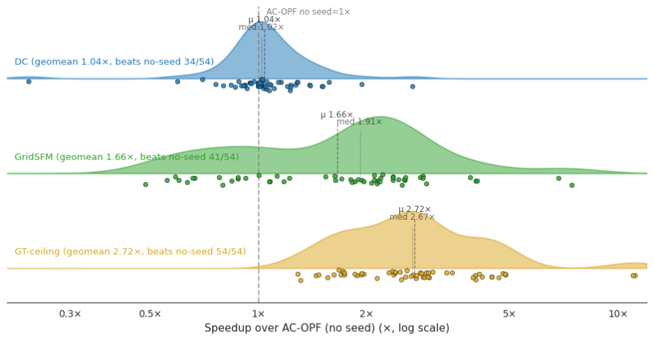
Our profile showed that GridSFM warm-start is 1.66× faster than cold start and 1.59× faster than DC-approximation warm-start (geometric means across the 54 grids test scenarios) and is faster than both baselines on 41 of 54 grids. The largest per-grid speedups exceed 7× over cold on the meshed transmission grids (Texas2k summer-peak, case2742_goc). DC-approximation warm-start, by contrast, is a wash on average across this broader grid mix (geomean 1.04× vs cold), DC saves on AC iterations on some grids and spends them rebuilding voltage/reactive on others.

The gap between the GridSFM distribution in Figure 7 and the GT-ceiling distribution (2.72× geomean) can be closed by improving GridSFM’s residual reactive-power and voltage prediction error, both targeted by the next release.

Generalization

We tested whether GridSFM-Open acts like a true foundation model by running it on a grid it had never seen before: the 6,470-bus case6470_rte from OPFData (opens in new tab), about 1.4× larger than any grid in training.

In a zero-shot setting, performance drops as expected. Cost error increases from 3.35% in-sample to about 14% on the new grid. Voltage predictions capture only about 27% of the true variation and appear nearly flat. The feasibility classifier flags every scenario as infeasible. Even so, the model still preserves the correct ordering of costs across scenarios.

With light fine-tuning, performance recovers quickly. After 10 epochs on 1,000 scenarios, cost error falls to 1.12%, voltage variation reaches 91% of the true signal, and feasibility detection becomes nearly perfect. An N-1 contingency split that was fully held out during fine-tuning matches the full-topology results within 0.2 percentage points on all metrics, showing that adaptation transfers across contingencies.

The model adapts even with very limited data. With just 10 scenarios, cost errors are 1.76% and feasibility detection exceeds 90%, with strong results already on cost and active power dispatch. Voltage magnitude is slower to recover and needs closer to 1,000 scenarios (see Table 1).

This test showed that GridSFM-Open already captures AC-OPF physics during pre-training. Adapting to a new grid is mostly a matter of calibration rather than relearning. The released checkpoint can therefore serve as a practical starting point for users to fine-tune on their own topology and tasks.

Fine-tune scenarios	Cost error	Feasibility Detection
0 (0-shot)	14%	0 (Collapsed)
10	1.76%	92%
100	0.88%	97%
1000	1.12%	99%

Looking ahead

Active directions for the next release:

• Generalization. Tighter accuracy on grids and operating conditions outside the training mix. The current out-of-distribution analysis is in the white paper.
• Continued accuracy improvements across all prediction channels, narrowing the residual gap between Figure 7’s GridSFM distribution and the gold GT-ceiling.
• Multi-snapshot extensions. Unit commitment (discrete on/off generator decisions across time), weather-conditioned scenario generation, dynamic-stability surrogates.

We previously released the GridSFM_US _Powergrid_dataset (opens in new tab). This release adds the first open AC-OPF model that supports multiple grid topologies, completing a stack of open topology data, open code, and open weights for ML-driven grid simulation and planning. We see it as a starting point for the community to build richer simulators, planning workflows, and decision-support tools without re-creating the data or the model from scratch. The applications we expect to see most leverage from are the ones where the cost of a single solve has historically forced cherry-picking: contingency screening, transmission expansion planning, demand-siting analysis, and resilience studies under extreme weather. 

Everything in the GridSFM-Open tier is released for research use today:

A note on GridSFM-Premier. The larger production-scale tier is not part of this open release. If you are interested in evaluating it, collaborating with us, or otherwise getting access, please contact us at gridFM@microsoft.com.

Opens in a new tab